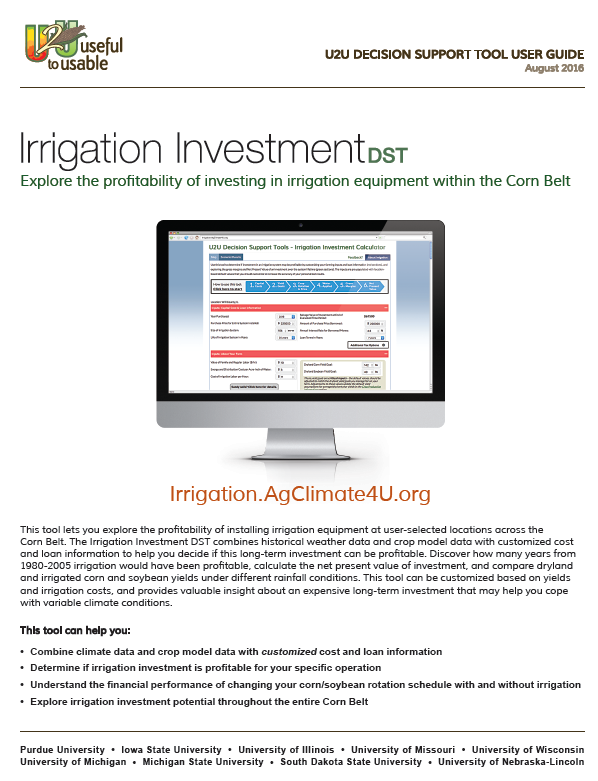
About the Irrigation Investment DST

Contributors

Jeff Andresen, Larry Biehl, Ben Gramig, Chad Hart, Dev Niyogi, Chris Panza, Molly Van Dop, Melissa Widhalm

Background

The U2U Irrigation Investment DST lets you explore the potential profitability of installing irrigation equipment at user-selected locations across the Corn Belt. Discover how many years from 1980-2005 irrigation would have been profitable, calculate the net present value of investment, and compare dryland and irrigated corn and soybean yields under different rainfall conditions. This tool can be customized based on yields and irrigation costs, and provides valuable insight about an expensive long-term investment that may help you cope with variable climate conditions.

Why Invest in Irrigation?

Irrigation is already well established throughout some portions of the Corn Belt. For example, in Kansas and Nebraska, the lack of rainfall, combined with temperate conditions and favorable soil, make these states prime targets for irrigation systems. Other areas in the Corn Belt are adopting irrigation not necessarily due to consistently low rainfall, but to cope with weather variability from year-to-year. The overall acreage covered by irrigation across the United States is growing and may prove to be beneficial for managing risk in corn and soybean operations.

Types of Irrigation Systems and Applications

Center pivot systems are the most common systems used for irrigating corn and soybeans across the Midwest. The Irrigation Investment DST provides default capital cost and loan values based on a center pivot irrigation system, covering approximately a quarter section (164 acres) of land. Other sizes and types of irrigation systems can be evaluated through the tool if all of the necessary cost and loan information for an alternative type of system is known.

Fact Sheets and Tutorials

Irrigation Investment_DST User Guide

Irrigation Investment_DST Training Webinar

Data Sources and Technical Details

The U2U Irrigation Investment DST helps you decide if investing in irrigation would be profitable based on location-specific data. The tool uses simulated historic yields (in the vast majority of counties) and irrigation water quantities for corn and soybeans based on climate model data and soil texture information. The tool also accounts for tax and loan information to identify whether irrigation investment is expected to be profitable over the useful life of the system. The data inputs and calculations used within the Irrigation Investment DST are described below.

Irrigation Investment Calculator Template

The Irrigation Investment DST framework is built on a spreadsheet-based decision support tool originally created by Roger Betz, with contributions from Lyndon Kelley and Dennis Stein, from Michigan State University Extension. The Net Present Value, tax information, and gross margin calculations were derived from the most recent version of this spreadsheet tool. Betz and Kelley were consulted during the development of the Irrigation Investment DST. The web-based implementation of the tool draws default values from crop simulations, USDA, and other sources described below based on the user selected geographic location.

Weather Data

The Irrigation Investment DST uses the Standard Precipitation Evapotranspiration Index (SPEI) to determine the occurrence of wet/normal/dry years throughout the period of record in a given location. The SPEI was designed by Dr. Sergio M. Vicente-Serrano, at the Instituto Pirenaico de Ecologia, Spanish National Research Council. It is an alternative measure to the more familiar Palmer Drought Severity Index (PDSI) that is specific to the individual location and tracks well with the PDSI. The SPEI is a normalized index used to measure precipitation extremes (wet and dry) based on both temperature and precipitation data. The SPEI is measured on a scale from -3 to 3, representing precipitation departures from average or “normal” conditions in terms of standard deviations. Values greater than or equal to 1 indicate wetter than normal conditions whereas values less than or equal to -1 indicate drier than normal conditions. Values between -1 to 1 are considered normal conditions. The SPEI was calculated using the ‘SPEI’ package in the statistical software program R, using the precipitation and temperature inputs to the crop model (see below), along with the Thornthwaite equation for estimating potential evapotranspiration. For the interested user, the SPEI based on historical weather observations at individual weather stations is available directly from the Drought Risk Atlas, a quality-controlled database developed by the National Drought Mitigation Center (NDMC) with funding provided by the NOAA Sectoral Applications Research Program (SARP).

The SPEI is calculated in the irrigation investment tool using the climate model data that were used to simulate dryland and irrigated corn and soybean yields (details below). Weather data from four climate models (GFDL, HadGEM, IPSL and NorESM) that best represent the 1980-2010 climate in the Corn Belt are the basis for the SPEI calculations and were used to drive the crop simulations with and without irrigation. The mean of the weather variables across the climate models is used in the SPEI calculations in the tool.

Crop Yield and Irrigation Application Quantity Information

For more information on yield, water application, or the user transformations, please contact Molly Van Dop (molly.van.dop@gmail.com).

To provide estimates of the profitability of irrigation investment, crop models and climate models are used to simulate yield and irrigation water quantity information for a location. Dryland and irrigated corn and soybean yields are based on simulations from the CERES Maize and CROPGRO models implemented in the parallelized version of the Decision Support System for Agrotechnology Transfer (pDSSAT) as part of the Agricultural Model Intercomparison Project, known as AgMIP. Irrigation water quantities are also outputs from these models. These values are default starting values, and are necessary to calculate the costs and revenues for a producer. This information is based on spatially-weighted county-specific weather and soil data, the yield values (and irrigation amounts) are most accurate if the user adjusts them to represent an individual field or local conditions, and can be customized in the tool after the defaults are loaded based on location.

Corn and Soybeans

The corn and soybean yield and potential irrigation water quantities in wet, dry, and average years are from the parallel DSSAT (pDSSAT) crop model simulations (mentioned above). These data were made available by Joshua Elliott at the University of Chicago. Crop growth simulations were run for each year from 1980-2005 using weather data from four different global climate models. The mean of the yield and potential irrigation quantities from the four climate models most consistent with the observed climate in the region are the default data presented and the economic basis for the calculations in tool. Soil data in the crop models are from the Harmonized World Soil Database (based on USDA soil data) for 55.5 x 55.5 km grid cells across the Corn Belt. The grid cell data were converted to county data by overlaying the county boundaries on the gridded data and calculating the area-weighted yield and irrigation amounts for each county. Based on the four month (May - August) SPEI each year, the yields and corresponding irrigation applications were sorted into wet, dry, and average years (using the method described in the “Weather Data” section). The average of the yields and water application amounts for the years in each weather type is taken as representative.

The simulated yields were bias-corrected following the procedure of Jagtap and Jones (2002) to minimize the root mean square error between the observed NASS county yield and the area-weighted simulated yield over the 1980-2005 period. This process was used to bias-correct all of the county area-weighted simulated crop yields in an effort to remove bias that may be present in the crop model or that is introduced when converting gridded simulation data to county data. Irrigated yields were bias-corrected using the same procedure if there was NASS county data available for irrigated yields (mostly in Kansas, Nebraska and South Dakota). Where irrigated county yield data are not available from NASS, the percentage yield difference between irrigated and dryland production from the 2013 USDA Farm and Ranch Irrigation Survey is applied to the mean county yield available from NASS to conduct the bias correction procedure. This information is the source of the default values, and any user adjustments to the defaults are used to update the default results, and may prove more accurate for a specific farm or field.

Variable Cost Information

Labor Information

Average wage rates for standard farm labor are based on the 2012 Kansas State University publication “Employee Wage Rates and Compensation Packages on Kansas Farms.” Average wage rates for irrigation-related labor are based on the state-specific 2013 Farm and Ranch Irrigation Survey (FRIS) values.

A report developed by Field to Market using USDA data through 2011 was used to determine the labor hours (without irrigation labor) required for each crop type. The 2014 Farm Management Guide from Kansas State University was consulted to determine the additional hours required for irrigation labor by crop type.

Crop Prices and Other Variable Cost Information

Crop prices are from the April 29, 2016 publication of “Agricultural Prices,” a monthly USDA document that includes the 2014-2015 marketing season prices for corn and soybeans. The 2015 Purdue Crop Cost and Return Guide was consulted for input cost information for many of the expenses the user encounters throughout the growing season, including seed, fertilizer, chemicals, fuel, repairs, crop insurance, and trucking costs (for both unirrigated and irrigated crops). There are two exceptions with respect to the irrigated crop values. First, the irrigated crop insurance values are from a Kansas State Research and Extension publication by Daniel O’Brien. Second, the repairs for irrigated crops use the Purdue Crop Cost and Return Guide repair amount added to the 2008 FRIS maintenance and repair cost per irrigated acre (Table 24). This allows for the irrigated acres to be subject to both the standard repair costs and the irrigation-specific repair costs. Additional input categories for irrigated crops come from the 2013 USDA Farm and Ranch Irrigation Survey data, such as the irrigation energy requirements (from Table 12).

Interpreting the Results

Gross Margin Calculations

The gross margin calculations reflect the profits associated with planting an acre of corn/soybeans on irrigated or unirrigated land, excluding any debt repayment costs of a loan for an irrigation system. The gross margins take into account the probability of a wet, dry, or average year occurring, along with the corresponding yields and variable costs.

The “Gross Margin Total” for unirrigated land (dryland crop) looks at the income the farmer would receive across their entire field from an unirrigated crop mix of corn and soybeans, using the expected yields and crop prices, and subtracting the variable costs. The crop rotation is taken into account as well. For example, if the rotation is said to be 50% corn and 50% soybeans, then half of the acres will be assumed to grow corn and half of the acres soybeans. The calculation for the “Gross Margin Total” for irrigated land is performed in the same way, except the variable costs and yields reflect irrigated corn and soybeans.

The “Total Gross Margin Benefit with Irrigation” is the difference between the “Gross Margin Totals” for irrigated acres and unirrigated acres. This benefit, divided by the acres of the area covered, is the “Gross Margin Benefit per Irrigated Acre.” A positive value indicates that, before taking the cost of the irrigation system into account, irrigation is profitable. A negative value indicates that even if the equipment was already installed and paid for, irrigation is not profitable.

Returns over System Lifetime Calculation

The “Net Present Value Discounted After Tax Cash Flow” calculates the discounted net benefits that investing in an irrigation system may (or may not, if negative) provide to the farm over the irrigation system’s lifetime. This takes the capital cost and loan information into account, along with the gross margins associated with irrigated and dryland acres. The process is a standard net present value calculation of the net benefits of irrigation over dryland production. This calculation can be customized using the “Capital Cost and Loan Information” and “Additional Tax Option” sections. Taking the full costs of the irrigation equipment into account, a positive Net Present Value suggests that, over the irrigation system lifetime, irrigation is more profitable than dryland production while a negative value suggests that irrigation investment is less profitable than dryland production.

When Is Irrigation Worth It?

The Irrigation Investment DST calculates the number of years (from 1980-2005) an irrigation investment would be profitable. The gross margins and Net Present Value are calculated individually, for each year in the historic time period, to see if the prospective investment would have paid for itself. This calculation does not take the salvage value of the irrigation equipment into consideration, but merely considers if the gross margins under each year's specific conditions would be great enough to cover the average costs and loan repayments for the equipment. Rather than averaging the yield, weather, and irrigation information (as done throughout the rest of the tool), by default this is calculated individually for each year, using the relevant crop model information. This is done to capture unusual conditions that may show the value (or lack thereof) for irrigation equipment in areas where it may not be profitable to otherwise irrigate. For example, if a location experienced significant drought conditions during two years of the historic period, it may have been profitable to own irrigation equipment during those two years, but when considered over the entire life of the irrigation system investment may not be a valuable investment. NOTE: If the user changes the default yield values or customizes the dryland yield goal, the calculation is altered and the mean yields by year type (dry/average/wet) are used to calculate the expected NPV instead of using individual yearly data from the 1980-2005 simulations.

Frequently Asked Questions

Note: All irrigation quantity defaults are based on simulations (pDSSAT model described above, except for a limited number of locations that are based on NASS data) and do not take into account any policy (regulations, water rights, etc.) or physical (access to groundwater) restrictions on the availability of water for irrigation.

What is the difference between the red and green section headings?

The red and green headings are visual cues to help the user easily identify if they are within sections dealing with data inputs (red) or tool results (green). Adjusting the values within the red sections may change the results displayed in the green sections.

So should I invest in irrigation or not?

After you’ve customized the input values (within the red sections) go to the “Results: Returns over System Lifetime” section and look for the “Net Present Value Discounted After Tax Cash Flow”. If this is a positive value, it means that the installation of irrigation equipment is profitable. If negative, installing an irrigation system is not profitable.

What should I do if I don’t know a specific input value?

All of the data input values are populated with default values that the user can adjust for customized results. There are many potential input values that can be customized. The Irrigation Investment DST is structured to easily see the most critical inputs to adjust. The input sections “Capital Cost & Loan Information” and “About Your Farm” have major impacts on the outcome of the tool, and tend to vary considerably between individuals. Other inputs are more difficult to customize and have less of an impact on the results. These inputs tend to be nested in the tabs containing the image of a gear, such as the “Additional Tax Options” box. Advanced users should feel free to adjust these as they see fit, but this is not necessary to successfully use the tool.

How is soil texture determined?

The crop yield and irrigation quantities in the tool are based on crop growth simulation models for corn and soybean. The soil in each location where simulations were conducted are based on the USDA soils database and may not represent an individual farm or field of interest to a user. Soil texture cannot be selected using the tool, but by adjusting the crop yields and irrigation quantities for your soils a reasonable estimate of the financial calculations should result. See sandy soil FAQ below for more related information.

How can the tool be used to evaluate irrigation on sandy soils?

The yield goal, and more specifically the dryland and irrigated yields for each crop in dry, average and wet years, can be used to evaluate investment on sandy soils if the user has appropriate values to enter for their location. Because a crop simulation has not been run for this customized set of conditions, the economic estimates should be evaluated carefully. Adjusting the yield goal and/or specific yields (see Inputs: Crop Production Information) without adjusting the irrigation water quantities required on sandy soils will not result in accurate economic calculations because the cost of additional irrigation water will not be accurate if default irrigation quantities are used with customized crop yields.

It is known that crop N uptake and soil moisture conditions are correlated, and the yield response to irrigation reflected by the default values for a user-selected location may not be comparable to yield response for other soil textures or conditions experienced on individual farms.

Do the results automatically update (or, do I need to push “calculate” somewhere)?

All calculations made inside the tool are updated as new information is entered—as soon as you type it into the tool. If you would like to return to the default values you can press the “Reset Inputs” button in the bottom-left corner of the Scenario/Results tab.

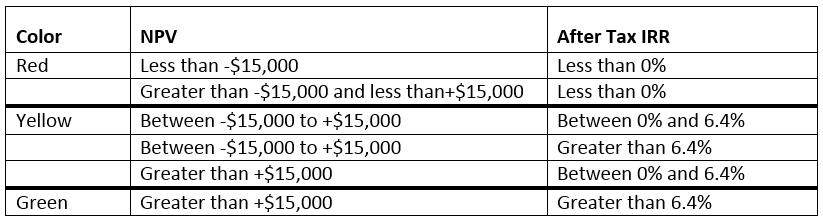
What does the color shading in the results (NPV, IRR) mean?

The Results: Returns over System Lifetime section reports the net present value (NPV) and internal rate of return (IRR) from the investment scenario constructed by the user. The left section of these results may be shaded one of three colors based on the level of the NPV and IRR. The colors and corresponding NPV and IRR values are summarized in the table below.

Why do irrigated soybeans seem to be more profitable than irrigated corn?

The crop growth simulation model for soybeans (CROPGRO, part of the DSSAT suite of crop models) has a programmed yield response to irrigation (and other inputs). The soybean yield response to irrigation is what is reflected in the default irrigated yields. In many locations, the profitability of irrigated soybeans has a large influence on the NPV calculation, and even if irrigated corn does not appear profitable on its own, irrigated soy is profitable. Local yield response to irrigation, for either corn or soybeans, may be different than the simulation results and yields should be adjusted to match local conditions.